Эта статья на русском: читать по-русски
The Problem With Optimizing One Variable
Supply chain design, at its core, is a minimization problem. The total cost of operating a supply chain network has three components:
Total Cost = Transportation + Fixed Facility Costs + Inventory Holding Costs
Or formally: TC = Σ c_ij · x_ij + Σ f_j · y_j + Σ h_j · I_j
Where c_ij is the unit cost of moving product from supplier j to distribution node i, f_j is the fixed cost of operating facility j, and h_j is the inventory holding cost at node j.
Most procurement teams minimize one term: the purchase price, which shows up as a component inside c_ij. Most logistics teams minimize another: the transportation rate per kilometer. Neither team is wrong. Both teams are solving a part of the problem while the total cost grows.
The place where this gap becomes expensive is geography.
A Worked Example: The Two-Supplier Problem
Imagine a food chain operating across a large country — 1,200 delivery points spread across twelve time zones. The company sources its highest-volume ingredient (let's call it Ingredient A) from two federal suppliers near the capital, who deliver into a central distribution center. From there, product moves to 17 regional cross-docking hubs, then last mile to restaurants.
The logistics structure looks like this for every kilogram of Ingredient A:
Supplier (capital region) → Central DC → Regional cross-dock → Restaurant
Each leg has a cost:
- Inter-DC transfer: $0.18/kg
- Central DC handling: $0.09/kg
- Long-haul transport to regional cross-dock: $0.10–0.42/kg (varies by distance)
- Last mile (~$0.15/kg): fixed regardless of supplier location
Now introduce a regional alternative — a supplier located 90 km from the Midwest cross-dock instead of 3,200 km away near the capital. Purchase price is identical.
The logistics cost change:
- Eliminates inter-DC transfer: −$0.18/kg
- Eliminates central DC handling: −$0.09/kg
- Eliminates long-haul from capital to Midwest: −$0.31/kg
- Adds short-haul from regional supplier to cross-dock: +$0.04/kg
- Last mile: unchanged
Net logistics saving: $0.54/kg. On 400 tons per year through that cross-dock, that's $216,000 per year — from one node, on one ingredient, at identical purchase prices.
Multiply across 8 cross-docks with similar geography and similar volumes, and the number becomes material.
Why the Math Isn't Linear
Here is where it gets counterintuitive. The savings are not proportional to distance. They follow a structure that supply chain network models call the facility location trade-off.
The formal version of this problem is called the facility location model — you're solving for the optimal placement of supply points to minimize total landed cost. The structure is a Mixed Integer Linear Program (MILP):
minimize: Σ_j f_j · y_j + Σ_i Σ_j c_ij · x_ij
subject to:
- Each node i must be served: Σ_j x_ij ≥ D_i
- A supplier j can only serve a node if it's active: x_ij ≤ M · y_j
- y_j ∈ {0,1} (binary: supplier is either in or out)
The insight the model reveals is this: as you add more regional sourcing points, transportation cost falls sharply at first (you're eliminating very long hauls), then flattens (you're adding suppliers in places where the haul was already short). Meanwhile, procurement complexity — qualification costs, safety stock requirements, relationship management — increases roughly linearly with the number of active suppliers.
The optimal point is not "as many regional suppliers as possible." It's the inflection where marginal logistics savings start to fall below marginal procurement overhead.
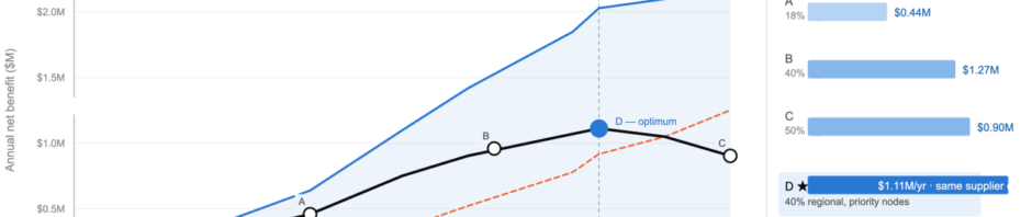
In the example above, this inflection appeared around a 60/40 split (federal/regional): enough regional volume to capture the largest logistics savings, not so much that you're chasing marginal gains at high coordination cost.
The Four Scenarios
Running the model across the 17 cross-docking nodes — using actual transport tariffs and node volumes — produces four scenarios depending on how aggressively you regionalize:
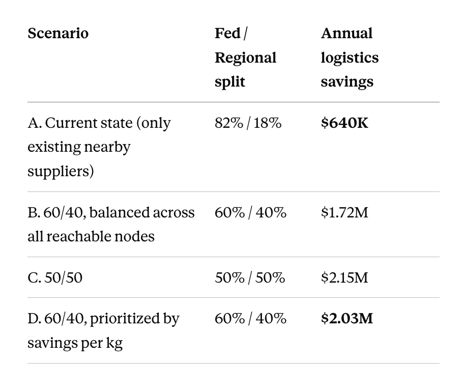
Scenario D is the practical optimum. It achieves the same regional volume share as Scenario B but concentrates that volume at the nodes with the highest per-kg savings — remote cross-docks where long-haul costs dominate. The result: $310K more in annual savings than the "evenly distributed" version at the same supplier count.
Scenario C saves $120K more in gross logistics savings than D, but requires moving 10 percentage points more volume to regional suppliers — additional qualification costs, higher safety stock at regional nodes, and ongoing relationship management overhead. Once that overhead is priced in (typically $130–150K/year for the extra supplier layer), D’s total cost of ownership is lower despite the smaller gross saving. The model optimizes logistics; the right answer optimizes total cost.
This is the stop density logic from route optimization, applied to sourcing geography: uniform distribution is never optimal. Concentration at high-value nodes always outperforms averaging.
The Constraint Nobody Models
Here's what the math cannot capture: supplier availability.
The model says you need regional suppliers near the Siberian cross-docks. The map shows three potential candidates. Two of them produce the wrong product format. One of them exists only in theory — they're a broker, not a manufacturer.
In practice, Scenario A (18% regional, $640K savings) is what you can start today, because the suppliers exist and are qualified. Scenario D ($2.03M savings) requires 12–18 months of supplier development: factory audits, quality validation, trial shipments, contingency agreements, dual sourcing minimums to keep the federal supplier engaged.
This gap — between the model's optimal and the operational reality — is where most regionalization programs stall. The economics are clear. The sequencing is the problem.
The practical approach is a three-tier rollout:
Tier 1 — Act now (suppliers qualified, economics strong): Nodes where regional suppliers already exist within 200 km. Start here in Q4. Run at ≥20% federal backup minimum to maintain optionality.
Tier 2 — Develop actively (economics strong, no supplier yet): Nodes where savings per kg exceed $0.35 but no qualified local source exists. These justify active supplier prospecting — send a procurement person there, not a price inquiry.
Tier 3 — Leave as is: Nodes where savings per kg are under $0.15. The procurement overhead of qualifying a regional supplier exceeds the logistics benefit. Keep federal sourcing, optimize terms instead.
The Second-Order Effect
There's an argument that rarely makes it into the regionalization business case, but probably should.
When a supplier knows that 80% of a buyer's volume is captive — that there's no credible alternative — they negotiate accordingly. Regional supplier development changes that. A qualified alternative in a given geography shifts the federal supplier from "sole source" to "preferred source." The negotiating dynamic changes before you've moved a single kilogram.
This is the sourcing leverage effect: developing a regional supplier is also a price signal to the federal supplier. Some portion of the total cost reduction in Scenario D comes not from logistics savings, but from purchase price improvement on the 60% that stays federal.
The model doesn't capture this. It should be in every TCO (Total Cost of Ownership) analysis.
The Connection to the Previous Problem
In the last article, I wrote about route optimization and the density trap: why sparse geographies cost more per delivery, not linearly, but following a square root relationship, as stop density falls.
Supplier regionalization is the same principle applied one tier upstream. When all your suppliers cluster near one city and your demand is distributed across a continent, you're paying a density tax on every kilogram of product you move. The algorithm can't fix it. The route optimizer can't fix it. The only fix is geographic repositioning of supply — which is a sourcing decision dressed up as a logistics problem.
The math connects: in distribution cost models, distance per stop grows with 1/√δ where δ is stop density. In supply network design, total transportation cost grows with the distance between supply nodes and demand nodes. Both frameworks say the same thing: geography is cost.
The question is whether you're treating it as a fixed constraint or a design variable.
When I think about what well-designed food supply chains look like at regional scale — whether in Central Asia, Southeast Asia, or across Eastern Europe — the common thread isn't sophisticated route optimization software or real-time inventory visibility. It's that someone, at some point, made the deliberate decision to move supply closer to demand. Not all the way. Not uniformly. But enough to change the shape of the cost curve.
That decision usually doesn't show up in a procurement savings report. It shows up in the P&L, two years later, as a structural margin advantage.
Originally published on .
