Before We Talk About Routes, We Need to Talk About the System
Most conversations about route optimization jump straight to the algorithm: VRP, Clarke-Wright, simulated annealing, machine learning. But there's a layer below that almost nobody touches in practice — and skipping it is why most optimization projects either underdeliver or quietly get abandoned.
That layer is the flow of the system itself.
Start with a simple observation. In any process — warehouse, truck fleet, distribution network — three things are always related: the number of items in the system at any given moment, the rate at which items move through it, and the time each item spends inside it. These three aren't independent. Change one and the others change too, mechanically, like a conservation law.
If your warehouse processes 100 shipments per day and each order takes half a day from receipt to dispatch, you will have, on average, roughly 50 orders in process. Not at every moment — at any given point the actual count can be higher or lower depending on arrival patterns and variability — but as a long-run average, this relationship is exact. It’s called Little’s Law (L = λW), and it holds in steady state regardless of the distribution of inter-arrival times or processing times. Want fewer orders in process? Either speed up throughput or shorten the processing time. There's no third option.
This seems obvious. And yet most distribution operations I've seen try to manage inventory and route timing as separate problems — without recognizing that they're expressions of the same underlying constraint.
The second thing that almost always gets missed is the bottleneck. Every system has one stage that limits the output of the whole chain. You can optimize every other stage to perfection; it changes nothing, because the output is capped by the slowest step. In a distribution context, this is often not the truck or the route — it's the loading dock, the dispatch window, or the inventory accuracy that makes loading possible in the first place.
I've seen cases where the routing was designed for 4 trucks and the network genuinely needed 4 trucks — but the warehouse could only load 2 per shift. The route plan was right. The bottleneck was upstream. Two trucks moved, two sat. And no amount of route re-optimization would have fixed it.
The third factor is variability. This one is the most underappreciated. When demand is unpredictable, when supplier lead times are uneven, when the gap between "what the system shows" and "what's physically in the warehouse" fluctuates — the effect on delivery costs is non-linear. Not just "higher on bad days." The relationship between variability and waiting time follows a curve: at low utilization, variability barely matters. As you approach capacity, the same variability causes costs to explode. This is why a distribution network that looks fine on average can generate emergency deliveries constantly — the averages are fine, but the peaks are brutal.
A Worked Example: The Two-City Problem
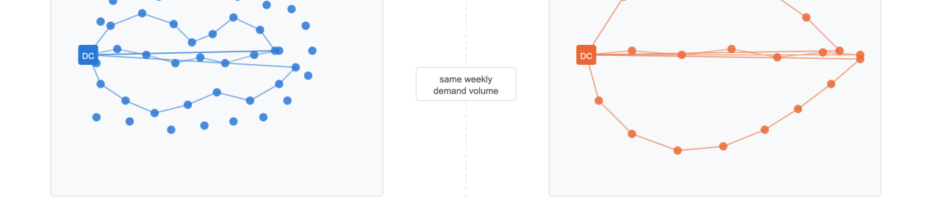
Imagine a food distribution company. Single depot. Two delivery regions.
Region A is dense: 50 restaurants within 30 km, all ordering daily. Region B is sparse: 20 restaurants spread across 150 km, ordering 3 times a week.
You want to estimate total fleet distance. Not optimize it exactly — just understand the structure of the problem before deciding how much to invest in fixing it.
For any one-to-many distribution network, the total distance across all vehicle tours has two components. The first is linehaul: how many trips from the depot to each region, multiplied by the round-trip distance. The number of trips depends on total demand volume divided by vehicle capacity — if total weekly demand for Region B is 40 pallets and your truck holds 10, you need at least 4 trips.
The second component is local routing inside each region: the distance the truck actually covers driving between stops. This part depends not on demand volume but on stop density — how many delivery points are packed into the area. Dense coverage means short loops. Sparse coverage means long detours between stops.
Here's what this reveals about the two regions. Region A has high density. Each truck trip is short. Linehaul is frequent but cheap per stop. Local routing is efficient. Total cost per delivery: manageable.
Region B has low density. Each truck covers a lot of ground between stops. Even if total demand is lower, the distance per delivery is much higher — not because the linehaul is longer (though it is), but because sparse stops mean inefficient local routes. Add the variability of 3x-per-week ordering patterns instead of daily, and you get inconsistent load factors on top of inefficient routes.
The trap is that most companies look at Region B's lower order volume and assume it's cheaper to serve. It often isn't. The sparse density makes local routing expensive in ways that don't show up in a simple cost-per-kilometer analysis.
And when Region C gets added — even sparser, even further — the economics get worse again, non-linearly. It's not that distance added to the network scales linearly with cost. The density effect compounds.
The Gap Between the Model and Tuesday Morning
Route optimization assumes the inputs are known. Demand at each stop, delivery windows, vehicle availability. The algorithm takes those inputs and finds a good solution.
The problem is that in many real distribution networks, the inputs aren't reliable.
Demand forecasting is informal. Stock counts are manual and sometimes days old. The warehouse team doesn't trust the system, so they plan by instinct. A region runs short on a key ingredient, a truck gets dispatched outside the plan at spot pricing, and the unit economics quietly deteriorate. The algorithm didn't fail — it never got clean data to work with.
Then there's the loading constraint. Routing software schedules routes based on vehicle count and capacity. It doesn't know that your dispatch dock has a 2-truck-per-shift limit. So the system generates a 4-truck plan. Two trucks load. Two wait. Half the routes don't run on time. Drivers learn that the plan is theoretical. They stop following it.
And then there's geographic expansion. Adding a new delivery region feels like adding new stops to the network. But as the earlier example shows, it changes the density of the whole distribution problem — and not in a linear way. What was manageable at 30 stops becomes chaotic at 80, not because the algorithm can't handle it, but because the organizational processes — verification, communication, exception handling — can't keep up.
What Actually Has to Come First
The diagnostic sequence I've come to use starts from the bottom of the stack, not the top.
Before optimizing routes, can you trust your demand data? Not "does a number exist in the system" — but "does the team making loading decisions trust it enough to plan against it?"
Before optimizing routes, is warehouse throughput a binding constraint? If the dispatch dock is the bottleneck, more sophisticated routing doesn't help. Fix the capacity limit first.
Before optimizing routes, do you have delivery confirmation data? Not just shipped — received, verified, timestamped, with responsibility assigned. Without this, the feedback loop that improves future route planning doesn't close.
Only after these three are solid does it make sense to invest seriously in route optimization tooling. The algorithm will do its job. The question is whether the organization can provide the inputs it needs and execute what it produces.
Originally published on .
