What the Model Was Actually Doing
Network design optimization is a well-specified mathematical problem. In its standard form, it's a Mixed Integer Linear Program:
min Σ f_j · y_j + Σ c_ij · x_ij
Subject to:
- Demand coverage: Σ_j x_ij ≥ d_i for all demand points i
- Capacity: Σ_i x_ij ≤ cap_j · y_j for all facilities j
- Binary: y_j ∈ {0,1} — a facility either exists or it doesn't
Where f_j is the fixed cost of operating facility j, c_ij is the cost of serving demand point i from facility j, and d_i is the demand at point i.
The model finds the configuration that minimizes cost — given f_j, c_ij, and d_i as inputs.
This is where the problem starts. Every single input is treated as a known constant.
The Constants That Aren't
Consider a company running its distribution through a 3PL provider — full outsource, 100% of volume. Leadership decides to evaluate bringing part of the network in-house: owned regional hubs that consolidate upstream supply and handle last-mile directly, with the 3PL managing the residual.
The MILP covers twelve scenarios, varying the share of volume through owned nodes from 5% to 80%. At the extremes:
- Low consolidation (5–20%): total cost higher than the pure 3PL baseline. Not viable.
- Medium consolidation (35–55%): near cost parity.
- High consolidation (60–80%): best-case savings of ~3% on a $35–40M annual logistics cost base — roughly $1.0–1.2M per year.
That's a real number. But it's the answer to the wrong question.
The right question is: what happens when the 3PL learns you're moving 60% of volume away from them?
The Parameter That Changes Everything
When you move 60% of volume in-house, the 3PL faces a choice: hold their tariff structure on 40% of remaining volume, or reprice to protect margin on a smaller base.
Run three scenarios: 3PL raises rates on residual volume by 10%, 15%, 20%. The ranking restructures entirely.
No tariff change: High consolidation (60–80%) wins. Saves $1.0–1.2M annually.
3PL raises rates 15% on residual: Medium consolidation (35–55%) — which looked like near-parity at baseline — becomes the actual winner. The "optimal" high-consolidation scenario loses most of its advantage to escalating residual cost.
3PL raises rates 20%: All scenarios above 35% consolidation look roughly equivalent. The ranking from the deterministic MILP is no longer meaningful.
One uncertain parameter — one plausible reaction from a counterparty — and the optimal answer changes entirely.
This is not a modeling failure. This is what happens when you solve a deterministic model over a stochastic problem.
The Formal Problem With Deterministic Optimization
MIT's supply chain network design curriculum distinguishes two approaches:
Deterministic optimization solves:
min TC(x, θ̄)
where θ̄ is a single fixed parameter vector — demand, costs, capacities — representing the expected state of the world.
Stochastic optimization solves:
min E_ξ[TC(x, ξ)]
where ξ is a random variable representing the true state of the world, and the expectation is taken over its distribution.
These are not equivalent. Two measures quantify the gap:
EVPI = min_x E_ξ[TC(x, ξ)] − E_ξ[TC(x*(ξ), ξ)]
EVPI — the Expected Value of Perfect Information — is the benefit you would gain if you somehow knew which scenario would materialise before making your network decision. Since perfect foresight can only help, EVPI ≥ 0. In networks with multiple interdependent nodes and external supplier behaviour, it is not small.
The more practically relevant measure is VSS — the Value of the Stochastic Solution:
VSS = E_ξ[TC(x̅(θ̅), ξ)] − min_x E_ξ[TC(x, ξ)]
where x̅(θ̅) is the solution to the deterministic model under expected-case parameters. VSS is the cost of pretending uncertainty doesn’t exist — the gap between what you pay when you run the deterministic model and implement its answer, versus what you pay when you model uncertainty explicitly. It is always ≥ 0.
The deterministic model gives you the optimal solution for a world that doesn't exist. The stochastic model gives you the best solution for the world that actually will.
What Simulation Adds That Optimization Misses
Instead of solving for the global optimum, the right approach shifts the question:
Not: What is the minimum-cost configuration?
But: Which configuration performs best across the full distribution of scenarios we might face?
This is a different problem. You're not minimizing cost — you're minimizing regret. The metric stops being E[cost] and becomes something like:
Minimax Regret: min_x max_ξ [TC(x, ξ) − TC(x*(ξ), ξ)]
Or in practical terms: which network configuration has the lowest P90 cost? Which configuration loses least when your assumptions are wrong?
In the example above, the scenario analysis covers:
- 12 network configurations (varying hub count and consolidation share)
- 3 tariff escalation scenarios on residual 3PL volume (10%, 15%, 20%) — 36 model runs in total
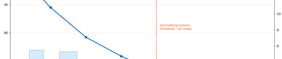
- Greenfield analysis: optimal network from scratch, testing configurations from 10 to 35 nodes
The Greenfield analysis produced an important finding: the mathematically optimal configuration required 35 nodes. But the cost difference between 20 nodes and 35 nodes was negligible beyond a threshold. There was no meaningful economic argument for the last 15 nodes. The optimization said "35." The scenario analysis said "stop at 20 and revisit."
Why Networks Built on Deterministic Optimization Become Fragile
The real cost of the deterministic approach isn't visible at implementation. It shows up two years later.
A network designed to minimize cost at one demand level and one tariff structure performs well in the scenario it was designed for. When actual demand deviates, when a key provider changes pricing, when a geopolitical event reroutes flows — the network has no resilience built in. Every departure from the design scenario becomes an exception that costs money to manage.
The supply chains I've seen fail under stress were almost always optimized, not robustified. They were efficient in the expected case and brittle in every other case.
The supply chains that held during disruption — sanctions, border closures, provider failures — were usually the ones designed with scenarios explicitly in mind: multiple sourcing options embedded, consolidation decisions made at a level where switching was still possible, provider dependencies managed as a risk variable rather than a cost variable.
Resilience is not a property you add to a network. It's a property you design in — or forfeit at the beginning.
The Practical Implication for Network Design Decisions
The shift I'd argue for isn't abandoning optimization. MILP is the right tool for what it's built for: finding the minimum-cost configuration given a parameter set. Run it. Run it across all twelve configurations and all three tariff scenarios.
What changes is what you do with the output:
- Don't pick the scenario that wins on the baseline. Pick the one with the best distribution of outcomes across scenarios — lowest worst-case regret (the minimax criterion), not lowest average cost. Minimizing average regret and minimizing average cost are mathematically identical; the meaningful distinction is between optimizing the expected outcome versus protecting against the worst-case outcome.
- Model the behavior of your counterparties, not just your own costs. In network decisions involving external providers, their response to your decision is itself a stochastic variable. Include it.
- Design for reversibility. The configurations that allow for phased deployment — start with 20 nodes, expand to 35 if economics hold — dominate configurations that require full commitment upfront. Optionality has value in network design exactly as it does in financial instruments.
- Set explicit review triggers. Not a fixed rollout plan, but a decision tree: if consolidation exceeds X% and tariff escalation exceeds Y%, move to next configuration phase. The roadmap is conditional, not linear.
The right answer in this example isn't high consolidation or low consolidation — it's medium consolidation with a phased expansion path: quick wins on existing network rebalancing, a starter hub configuration, a formal decision gate at 12 months — with explicit conditions that trigger or prevent the next phase.
Not an optimal network. A network designed to stay good across a range of futures.
A Note on the Digital Twin
The scenario approach only becomes tractable when the model is calibrated against actual operational data — real transport legs, real handling rates, real demand patterns. A digital twin built on a full year of shipment history turns "run 12 configurations × 3 tariff scenarios" from a research project into an afternoon. The upfront investment is in building the twin. The insight generation scales almost for free.
The failure mode I see most often in network design projects isn't a bad model. It's a good model used to answer one question instead of twelve. The model gets built, the optimal answer gets reported, and the decision gets made — without ever asking what that answer looks like when one key assumption is wrong.
Build the twin. Run the scenarios. Then decide which network you want to operate.
The example is illustrative, constructed to reflect the structure of real network design decisions across multi-cluster QSR and retail distribution contexts. The framework for stochastic network optimization draws on coursework from the MITx MicroMasters in Supply Chain Management.
Originally published on .
