Your demand is not random. It is reading the weather forecast
Picture a weekly supply review in late June. Last week a heatwave pushed one region above 30 °C for five days. Cold-beverage bases and dessert mixes ran out in a third of the outlets served by one cross-dock hub. The stock existed in the network, just not where the heat was.
The planner shows the forecast: a four-week average of the same weekday, the default setting in the replenishment system. It predicted a normal July week.
Someone asks the obvious question: “Couldn’t we have seen this coming? The heatwave was on every weather app for a week.”
The usual answer is “summer demand is volatile”, followed by a request for more safety stock. More stock is the expensive answer. You pay for it all season, it fills chilled space, and for short-life products it ends up written off when the weather turns.
The better question is this: how much of that “volatility” is explained by something we can see days in advance, and what is it worth to use it?
Noise is what you cannot explain
A swing in demand that follows the temperature on the same day is not noise. It is a variable you left out of the model.
That distinction matters for money. Safety stock is supposed to protect you against uncertainty. When you hold it against a swing you could have predicted, you are not paying for uncertainty. You are paying for ignorance.
For cold beverages, desserts and other temperature-sensitive lines, the weather is the single largest driver of day-to-day demand. Yet in most restaurant networks, these categories are still forecast as if the weather did not exist.
The Asymmetry That a Single Slope Misses
Even teams that do use temperature usually add it as one slope: “sales rise x% per degree.”
That fails because the response is not symmetric. Analysis of beverage sales across climate zones shows a clear pattern:
- Above the threshold: +12–13% demand per degree — heat triggers thirst-driven, impulsive purchases with no natural ceiling.
- Below the threshold: −5–6% demand per degree — cold mostly removes casual traffic and leaves loyal core demand alone.
A single slope averages these two regimes. It ends up too steep in winter and too flat in summer, which means it under-forecasts exactly the days that cause stock-outs.
The Model: A Hinge, in Logs
The fix is a regression with a bend in it. Model the logarithm of daily demand:
ln(y) = α + β_hot × max(T − τ, 0) − β_cold × max(τ − T, 0)
+ weekday effects + γ × promo + trend + ε
Where:
- y is daily demand for one product at one cluster of outlets
- T is the daily mean temperature (for forecasting: the weather forecast, not the actual)
- τ is the threshold where behaviour changes regime
- β_hot and β_cold are the slopes above and below the threshold
- γ is the promotion lift; ε is the noise we cannot explain
Working in logs does two useful things. Effects multiply, as they do in reality: a hot Saturday with a promotion is “hot × Saturday × promotion”, not a sum. And every coefficient reads directly as a percentage — a β_hot of 0.12 means e^0.12 = 1.127, so +12.7% per degree.
For a given threshold, this is ordinary least squares. The threshold itself is found by brute force: fit the model for every candidate from 10 °C to 28 °C in half-degree steps and keep the one with the lowest error or lowest AIC. If the hinge does not beat a single slope, your category does not have the asymmetry — and you have learned something too.
A Worked Example
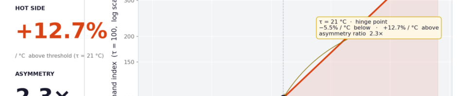
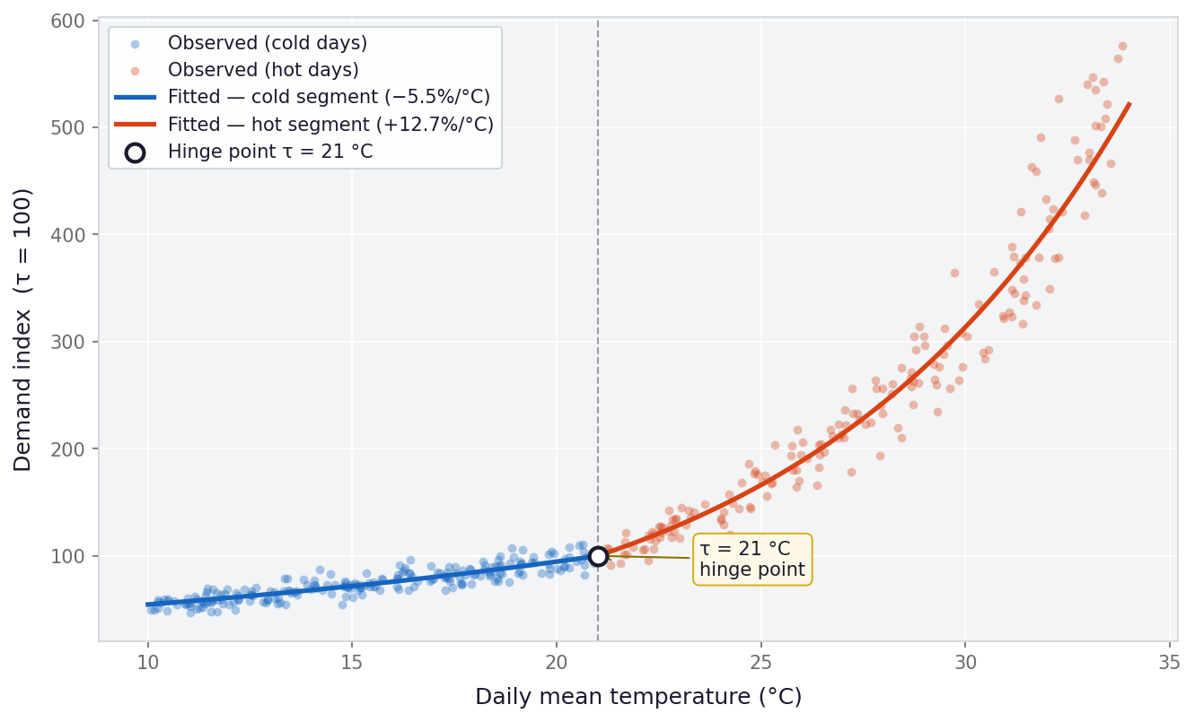
To make this concrete, I simulated two years of daily data for one hub of a restaurant network: about 70 outlets in a temperate climate, one cold-beverage base sold in cases. The data are calibrated to a real-world QSR network structure, with a threshold of 21 °C, +12.7% per degree above, −5.5% per degree below, weekday effects, promotions and a 3% annual trend. In July of year two there is a twelve-day heatwave peaking at 32.4 °C, hotter than any day in year one.
Setup: fit on year one, test on year two; daily review, 5-day lead time (6-day exposure window); 99.3% service target (z = 2.44); $25 per case, 25% annual holding rate. Weather forecast error: 1.5 °C one day ahead, rising to 3.0 °C six days ahead.
What the model recovered from one year of data:
- Threshold: 20.5 °C (true: 21 °C)
- Above threshold: +12.6% per degree (true: +12.7%)
- Below threshold: −5.6% per degree (true: −5.5%)
- Explained variance in log demand: 97.7%
Then I compared day-ahead forecasts on year two against what replenishment systems typically use, and against gradient boosting on the same inputs.
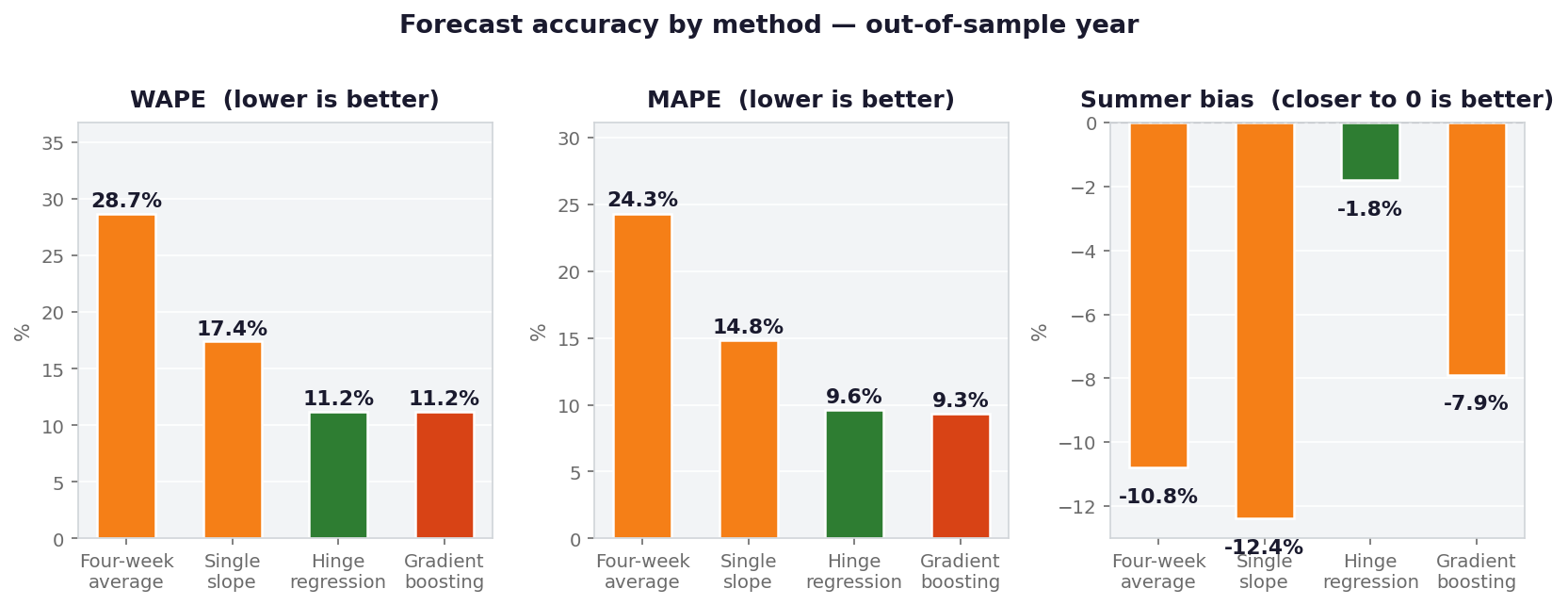
Three things stand out.
The default is worse than doing nothing clever. The four-week same-weekday average has a WAPE of 28.7%. Simply copying yesterday’s demand gives 15.1%. In a weather-driven category, last month is the wrong reference. Its annual bias looks harmless only because it lags in both directions: −10.8% as spring warms up, +5.8% in winter.
The single slope looks fine on MAPE and fails in summer. It under-forecasts June to August by 12.4% — exactly the asymmetry, ignored.
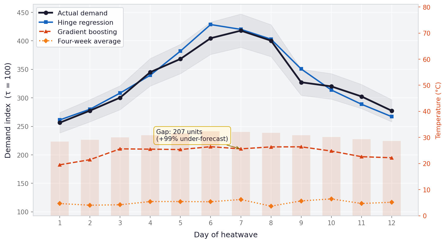
Machine learning ties on accuracy and loses on bias. Tuned gradient boosting matches the hinge model on WAPE (11.2%) and even edges it on MAPE. On a standard dashboard, it wins. But it under-forecasts summer by 7.9% and the heatwave by 14.5%. The reason is structural: a tree model predicts a constant beyond the hottest day in its training data. The hottest day in year one was 30.2 °C. The heatwave reached 32.4 °C. The model flattened exactly when demand accelerated.
Why Bias Matters More Than MAPE
MAPE and WAPE tell you how big your errors are. Safety stock can absorb errors of a known size. What it cannot absorb is a forecast that is consistently on one side.
In the example, gradient boosting needs a summer buffer of 381 cases. But its −7.5% bias over the six-day window quietly eats 73 of them. Effective cycle service falls from the 99.3% target to about 97.6% — in the season when stock-outs are most visible.
Report bias next to MAPE. Report it by month and by temperature band. A forecast that is 10% wrong in both directions is a safety-stock problem. A forecast that is 5% wrong but always low is a service problem.
From Forecast Error to Working Capital
The safety-stock formula is the familiar one:
SS = z × σ(R+L) ≈ z × σ_d × √(R + L)
Where z is the safety factor, R the review interval, L the lead time, σ_d the standard deviation of daily forecast error.
Two lessons from the example.
First, σ is seasonal. For the hinge model, the summer error is about five times the winter error in cases. A safety stock calibrated on the annual σ would deliver only about 92% service in summer and hold 2.9 times the stock needed in winter. Temperature-sensitive items need season-specific safety-stock tables.
Second, the √(R+L) shortcut understates weather-driven risk. Weather forecast errors get worse with horizon and persist from day to day. Measured directly over the six-day window, the hinge model’s summer σ is 41% higher than √6 times its daily σ. For the four-week average it is 2.2× higher. Measure σ over the full window instead of scaling it.
With that done, moving this SKU at this hub from the four-week average to the hinge model cuts the average safety stock from 334 to 127 cases. In summer the buffer drops from 7.8 days of demand to 1.8 days — about $5,175 of working capital for one SKU at one hub.
Scale it to four temperature-sensitive SKUs at 17 hubs: ~$352,000 released, ~$88,000 a year in holding cost, before counting chilled space and write-offs. Service goes up, not down.
The Weather Forecast Is Now Your Biggest Error
Once the model is in place, the largest remaining source of error in summer is not customer behaviour. It is the weather forecast.
With perfect temperature knowledge, the summer six-day σ would fall from 117 to 40 cases. Weather-forecast error accounts for about 88% of the summer error variance. At 12.6% per degree, a forecast that is 2.5 °C too hot inflates the demand forecast by about 35%.
Practical implications:
- Track your weather forecast error per location and per horizon, as carefully as your demand forecast error.
- Archive the forecasts as issued, not only the actual temperatures. Most teams keep only actuals and cannot fit on what they really knew.
- Know what a better weather source is worth. In the example, moving from a 1.5–3.0 °C error to a 1.0–2.0 °C error saves about $63,000 of working capital across 68 SKU-hubs.
A technical note: because the hot side is convex, a noisy weather forecast biases demand upward. With a 3 °C error, that bias is about 6.7% on hot days. Fitting the model on forecasts as issued fixes most of it.
When to Use Machine Learning
This is not an argument against gradient boosting. Use it when there are many interacting drivers — temperature, humidity, holidays, local events, delivery-app outages — and enough pooled history to learn them. When you do, constrain it to be monotonic in temperature, and feed it features that extrapolate, such as the hinge terms themselves.
Use a regression when the drivers are few, the shape is known, the business needs coefficients it can read (“+12.6% per degree”), and the forecast must work outside the range of history. A record heatwave is always outside the range of history.
One warning on flexibility: the deep-tree version in the test reproduced the training year almost perfectly and was worse on the test year than the tuned version. A model that is perfect in-sample has memorised the noise.
Five Questions for Monday
- Which of our categories respond to temperature, and have we tested for a threshold and asymmetry, not just a single slope?
- Do our forecast reports show bias, by month and temperature band, next to MAPE?
- Is safety stock calibrated on seasonal σ measured over the full review-plus-lead-time window, or on one annual number?
- Do we archive the weather forecasts we used, and do we know their error by horizon for our locations?
- If a new model beats ours on MAPE, how does it behave on days hotter than anything in its training data?
Demand in temperature-sensitive categories is not random. It is reading the weather forecast. The only question is whether your planning system reads it too.
Originally published on .
