Эта статья на русском: читать по-русски
Most managers intuitively believe that reviewing inventory less frequently saves time and cost. Mathematically, it does the opposite — and the delta compounds across every SKU in your network.
There's a question I ask every procurement or operations manager I work with when we first discuss inventory policies:
"How often do you check your stock levels?"
The answers vary — weekly, twice a week, monthly. Very rarely: daily.
The follow-up question is the one that tends to change the conversation: "Do you know how much that review frequency is costing you in frozen working capital?"
Most don't. And the reason is that the relationship between review frequency and safety stock is non-linear, counterintuitive, and almost never made explicit in the systems that generate replenishment orders.
I first encountered the formal framework for this in Dr. Chris Caplice's inventory management courses at MIT. The mathematics is clean. The practical implication, once you run it against a real network, is anything but small.
Two Policies, One Supply Chain
Inventory theory offers two fundamental approaches to replenishment:
Continuous review — (s, Q) policy
You monitor inventory in real time (or daily). When stock falls to a reorder point s, you trigger an order of fixed quantity Q. The inventory position is checked continuously; the trigger is automatic.
Periodic review — (R, S) policy
You check inventory every R time units (weekly, bi-weekly, monthly). At each review, you order whatever quantity brings you up to a target level S. Between reviews, you don't look — and don't order.
At first glance, periodic review seems simpler and cheaper to operate. You batch the cognitive and administrative work into a fixed cadence. One review per week instead of seven.
The problem is what happens during the interval between reviews.
The Mathematics of Uncertainty Over Time
Safety stock exists to absorb demand variability during the period when you cannot respond. Under continuous review, that period is the lead time L — the gap between placing and receiving an order. If demand spikes unexpectedly, you placed your order at reorder point s, and the goods arrive in L days.
Under periodic review, the exposure window is longer: R + L. If demand spikes the day after a review, you won't notice until the next review R days later, and goods won't arrive until L days after that. You are blind for R days.
The safety stock formula captures this directly:
Continuous review:
SS_c = z × σ_d × √L
Periodic review:
SS_p = z × σ_d × √(R + L)
Where z is the service-level coefficient, σ_d is demand standard deviation per time unit, L is lead time, and R is the review interval.
The ratio between them:
SS_p / SS_c = √((R + L) / L) = √(1 + R/L)
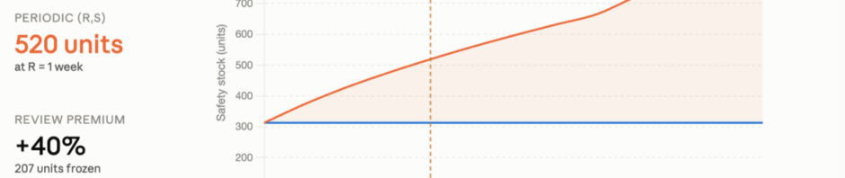
This is the cost of infrequency. When review interval R equals lead time L, periodic review requires 41% more safety stock than continuous. When R is twice L, the premium rises to 73%. The relationship grows with the square root, so it never becomes catastrophic — but it never disappears either.
A QSR Illustration
Let me make this concrete with an abstracted example from a distributed beverage franchise network.
Ingredient A — a temperature-sensitive beverage concentrate delivered to five regional warehouses across different climate zones.
Parameters:
- Weekly demand forecast: 650 units
- Demand standard deviation (empirical, weekly): 170 units
- Lead time: 4 days (0.57 weeks)
- Target service level: 99.3% → z = 2.44
- Review interval options: daily (continuous) vs weekly (R = 1 week)
Safety stock calculations:
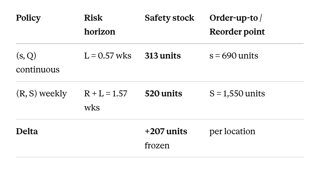
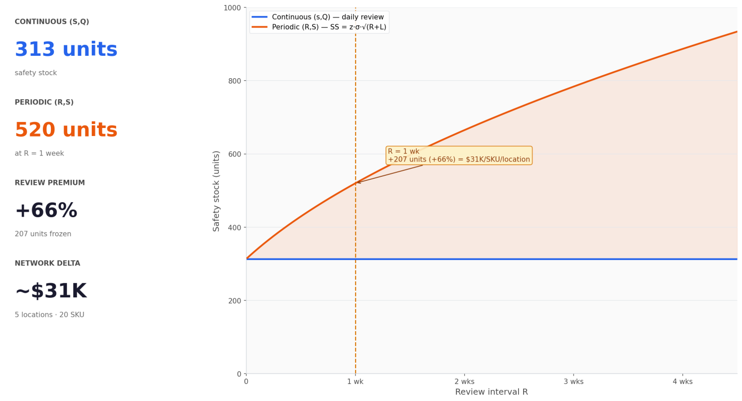
207 units per location. At a unit cost of $1.50, that’s $310 in permanently frozen working capital per SKU per warehouse — capital that generates no revenue, occupies shelf space, and in the case of perishable ingredients, creates write-off risk.
Across 5 locations and 20 temperature-sensitive SKUs:
207 × $1.50 × 5 × 20 = ~$31K tied up in review-interval inventory
Not in safety stock against real demand uncertainty. In safety stock against the fact that you didn't check yesterday.
The Temperature Wrinkle
Standard inventory models assume demand variability is stationary — σ_d doesn't change month to month. For most QSR categories, this is approximately true. For cold beverages, it's demonstrably false.
Empirical analysis of beverage sales across climate zones shows a well-documented asymmetry: demand rises roughly 12–13% per +1°C above a threshold, but falls only 5–6% per −1°C below it. The mechanism is physiological and behavioral — heat triggers impulsive thirst-driven purchasing with no natural ceiling, while cold primarily affects casual traffic without eliminating loyal core demand.
This asymmetry has two implications for policy choice:
First: σ_d is seasonal. Your winter σ_d and summer σ_d are different numbers. A safety stock formula calibrated on annual average demand variability will be systematically under-stocked in July and over-stocked in January.
Second: the value of continuous review is higher in summer. When a heat event hits unexpectedly, continuous review catches the inventory drawdown in real time and triggers a reorder within one review cycle (one day). Periodic review — if you're two days past your weekly check — won't trigger a reorder for five more days. Five days at +12%/°C demand acceleration can exhaust a full week of safety stock.
In practice, this means that the policy choice is not static: a beverage operation that runs periodic review in winter may need to shift to continuous in summer, or build season-specific safety stock tables for each temperature cluster.
The Network Aggregation Problem
One more layer that matters at scale: safety stocks don't aggregate linearly.
If you have five warehouses serving different demand regions, the naive approach is to calculate safety stock per warehouse and sum them. But this overstates the true buffer required by the central stock, because fluctuations across regions are partially independent — when the south runs hot, the north may be cool.
The correct aggregation for independent demand:
σ_total = √(σ₁² + σ₂² + σ₃² + σ₄² + σ₅²)
Not Σσᵢ. For five equal warehouses with σ = 170 each:
- Naive sum: 5 × 170 = 850 units
- Correct aggregation: √(5) × 170 = 380 units
The difference — 470 units — is the risk pooling effect of centralised visibility. It is only achievable if you can see all five locations simultaneously and reallocate in real time. Which, again, requires continuous rather than periodic monitoring.
When Each Policy Wins
Neither policy is universally superior. The choice depends on four parameters:
Use continuous (s, Q) when:
- Items are expensive or perishable (high cost of overstock)
- Demand is volatile or weather-driven (high σ_d, non-stationary)
- Your WMS or ERP provides real-time inventory visibility
- The product's contribution to stockout cost is high
Use periodic (R, S) when:
- Items are cheap, non-perishable, with stable demand
- Supplier imposes fixed delivery schedules regardless of order timing
- IT infrastructure supports only batch-mode stock counting
- Multiple SKUs can be logically batched in one review cycle
In practice, the real bottleneck is usually operational, not mathematical. The QSR industry historically runs periodic review because physical stock counting was manual. As ERP and WMS systems with real-time scan-in capability became standard, the cost of continuous review dropped to near zero — while the working capital benefit of the shift remained constant.
The question has changed from "can we afford continuous review?" to "do we know what periodic review is costing us?"
The Decision Framework
Before choosing a policy, calculate the cost of infrequency for your highest-value SKUs:
Step 1: Estimate σ_d from historical demand data (separate summer and winter datasets if the category is temperature-sensitive).
Step 2: Calculate SS_p and SS_c for your current lead time and review interval.
Step 3: Multiply delta by unit cost and number of locations.
Step 4: Compare against the operational cost of shifting to daily review.
For most QSR categories, step 4 produces a number close to zero — modern systems review automatically. The delta in step 3 is pure working capital freed.
Closing
The review policy embedded in your replenishment system is one of the most invisible levers in supply chain finance. It doesn't appear in a P&L line. It doesn't generate a variance report. It quietly determines how much working capital is parked in warehouses against uncertainty that your system could be monitoring in real time.
The formula is simple. The implication is not small.
If you're running weekly reviews on temperature-sensitive perishables across a distributed network, you're not just accepting operational simplicity. You're accepting a structural overstock position — and its associated working capital cost — as a permanent feature of how your supply chain works.
It doesn't have to be.
Originally published on .
